The first part of my series around Power BI, Excel & Dynamics GP begins with some of the basics, and a way to start learning Power Query, starting from scratch.
From my experience, an audience that is often overlooked is users who want to learn more or improve their skills but don't know where to start, and everything they find starts at a point they don't understand or can't get to. For example, this post starts without getting into directly accessing data from SQL, which admittedly adds a level of complexity that some users have trouble getting past. For most of the rest of this series, I will be accessing SQL data as that's more efficient, but in this one, I'm using SmartList exports to make the learning more accessible.
This is post #1 of the series, aside from the introduction post here. In this post, I'm using the context of Dynamics GP to make a "real world" example with Accounts Payable data.
Overview
This post will cover setting up a SmartList favorite (to be able to re-export newer data later in the same format), exporting it to Excel, saving it and then referencing it as a data source. This isn't about "export then manipulate into something", it's about exporting and reading the file as a quasi table/database to reference.
Using Power BI or Excel we can read those spreadsheets as a data source, and as newer versions are exported and saved over the original file, the workbook can be refreshed and/or the PBI file can be refreshed and it updates with that new data. Reading GP (SQL) data directly is "better" from an efficiency point of view, but it adds a layer of complexity around data access that isn't relevant to the core concepts behind getting started with some core skills.
The scenario
Let's say a request came in to put together some metrics on Accounts Payable activity, how many invoices are processed per month or quarter, how many payments are processed etc. That will be the basis for my example.
Step 1 - SmartList favorites
First, I will start with "Payables Transactions", which is an "out of the box" SmartList that comes with Dynamics GP. If access to that SmartList isn’t possible, the "Receivables Transactions" SmartList has fairly similar columns and the concepts are similar between A/R and A/P.
- Open SmartList and go to Purchasing > Payables Transactions
- Click on either the SmartList object name itself or the * to get the default set of columns
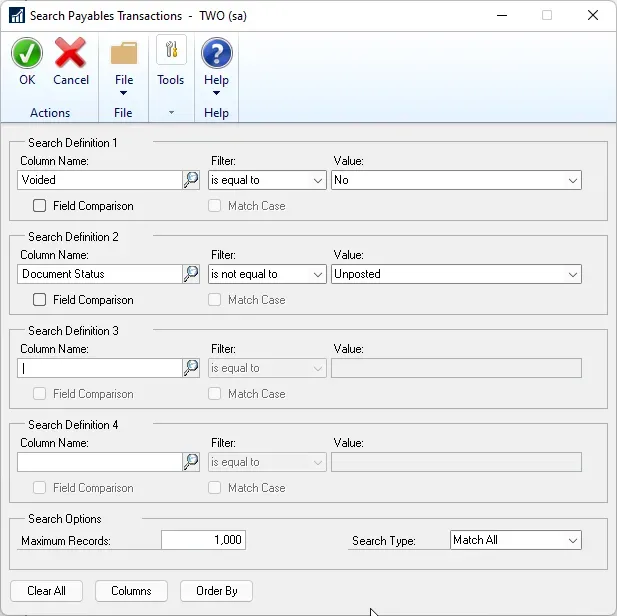
- Let's filter the list first under Search [Footnote 1]
- Voided is equal to No
- Document Status is not equal to Unposted
- Posting Date is greater than ** [Footnote 2]
- Add the necessary columns:
- Click on the Columns button on the toolbar
- Click on Add. [Footnote 3]
- Here are the columns I've included: Voucher Number, Vendor ID, Vendor Name, Vendor Class, Vendor Status, Document Type, Document Number, Document Date, Posting Date (aka GL Posting Date), and Document Amount.
- Don't worry about the order of the columns, that can be altered in Power Query.
- Save as a Favorite:
- Click on Favorites
- Give the list a name. I called mine "PBI".
- Optional: Set Visible To
- Click Add > Add Favorite
- Export the list to Excel
Footnotes (tips)
- [1] to search for a column not in the displayed column list, in the lookup for columns, click at the top where it says "Selected Columns" and choose "All Columns". The fields I note are not typically on the default SmartList set of columns but they will be listed under All Columns. This particular SmartList contains most of the fields from the Vendor tables which helps us in this case to include some basic vendor information.
- [2] Fabrikam's data is awful and limited. There are fewer than 1000 records in my data and the dates don't make a lot of sense compared to what normal production data may look like. In a real scenario, I might want to export data from the last 2-3 years to compare year-over-year transaction volume. With Fabrikam, I exported everything. Remember to change the Maximum Records to more than 1000 if there are a lot of records to deal with.
- [3] To select more than one column at a time, hold down the CTRL key and click the columns (for multi-select).
Step 2 - Saving the export
Now that the list has been exported, resist the temptation to format them or change them in any way! I will be using this as a data source, so I do not want to touch or change anything. The goal is to leave them as close to their raw format as possible so that each export is identical in layout. Power Query will expect the same filename, same path, and same tab name to read "updated" versions of the file when newer versions are exported in the future.
If others want to "refresh" this report, save it to a location those users have access to and save the spreadsheet into a folder with a meaningful name. The spreadsheet can be closed now, it's just a data source, I will not be opening it again!
Step 3 - Power Query
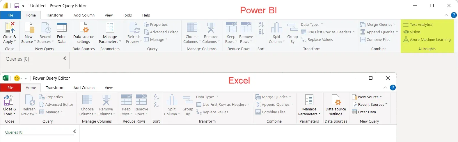
Before I begin, here are the two layouts of Power Query side by side, in Power BI and Excel. Some things are in a different order on the Home toolbar and a few things are only in Power BI (AI Insights and a couple of items on other menu tabs).
Open Power BI or Excel, and launch Power Query. For this post, I will use Excel. From what I described, technically Power Query does not need to be opened first, but for this example, I will start by going into Power Query first. How to get into Power Query differs slightly between the two applications.
- In Excel, go to the Data menu > Get Data > Launch Power Query Editor
- In Power BI, click on Transform Data > Transform Data
Here are the steps to get the data into Power Query:
- Look for the New Query section of the menu, click on New Source > File > Excel Workbook
- Browse to the folder where the spreadsheet was saved and select that file.
- The next window will have something like the picture below.
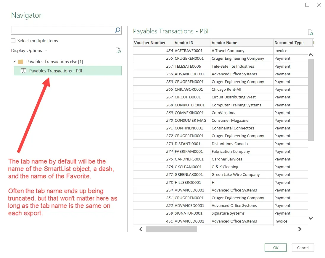
- The tab name is the name when the data is exported from SmartList. Part of the tab name is the name of the favorite so the important part is to use the same favorite to export each time.
- In this scenario, there should only be one tab in the workbook if it was saved right after exporting from SmartList. If using a different workbook that had multiple tabs and/or tabs with tables in them, it would show all of that with a slightly different icon for a tab of data vs. a table of data on a tab.
- Click OK.
Power Query Basics
The way Power Query works is it tracks each step performed on extracting or transforming the data, and they are listed on the right-hand side under the heading of Applied Steps. Each time the data is refreshed, Power Query repeats those same steps in the same order, eliminating the need to redo the steps manually every time. This is the beauty of using it for things where the same things need to happen over and over, and it's a lot easier than trying to use VBA to program a macro!
Don't be afraid to click on a prior step to see what it did, or what the data looked like after that step, before any other step being performed. The first step in my example is "Source". The other 3 steps were done automatically based on the type of data source I selected. Click on Source, for example. Mine looks like this:
- In the "formula bar", the pathname to the file is visible. This is where it would be updated if the source file needed to be moved somewhere else. (Two options for changing the file name or path are to edit in the formula bar or click on the Gears icon beside the word Source under Applied Steps, and browse to the new file/location).
- In the "table", certain parts of what it was reading from Excel such as the tab name will be recognizable.
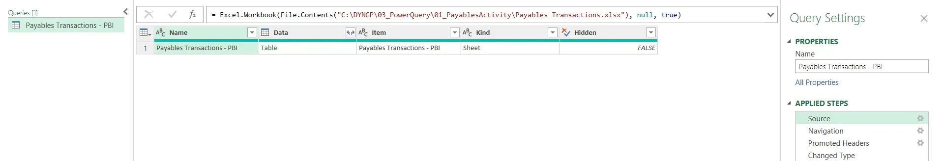
The Navigation step is essentially the act of drilling into the "table" of data on the tab we selected. At that point, it drills into it without recognizing the column names, and the headers will display as Column1, 2, 3, etc.
Promoted Headers is a step to tell Excel that the first row of data is the column names. This is a common step that could be added manually (in other scenarios) but done automatically in this case.
Changed Type is where Power Query has looked at the data and guessed what type of data is in each column. This may be right, or it may be incorrect. That is the first thing that I will review and in most cases, the first thing I do with a file no matter what the data source is.
Extract, Transform & Load (ETL)
What I've done so far is the very first part of ETL, extracting the data. The next step is to transform the data. This post is just scratching the surface of what could be done next, and in future posts, I'll go deeper into tips and tricks.
Review Data Types
- Some changes are required. For the first time through this, I'm going to delete the Changed Type step and redo it from scratch just to show how it is done. To delete a step, click on the X that appears when hovering over the step name. Now everything has ABC123 in the upper left-hand corner. That symbol means a data type of “any”. Even if the data “looks fine”, we want to set the data type to the right type for the data in the field so that PQ doesn’t guess wrong at some future date down the road.
- Click on the Transform menu tab, and change the following:
- Select all the following columns that are text and then choose Text in the Data Type menu on the toolbar.
- Voucher Number, Vendor ID, Vendor Name, Document Type, Document Number, Document Status and Vendor Class.
- TIP: columns can be multi-selected by holding down the CTRL key as they are clicked.
- The symbol on each should now be ABC.
- On Document Date and Posting Date, set as Date.
- On Current Trx Amount and Document Amount set as Currency.
- Select all the following columns that are text and then choose Text in the Data Type menu on the toolbar.
- When this is done, all of those changes were the same type of change, so there is only one “step” added and it's called Changed Type.
- TIP: to change the Data Type of one column, click on the symbol on the left corner of the column name to see the data types and choose the correct one.
Trim excess spaces
This step is specific to GP data because Dynamics GP text fields contain trailing spaces which are a pain to deal with in some cases, so trimming them is good practice. "Trim" means removing empty spaces at the beginning or end of a string.
- Select all of the Text (ABC) columns in the source (the same columns we set to Text above)
- On the Transform menu, click on Format then Trim.
Flip the document amount
This step is also somewhat specific to Dynamics GP. Dollar amounts in most tables are not based on the type of document, i.e., they are all displayed as positive amounts with a separate Document Type column. What this means is out of the box, a column of transactions cannot be “summed” to determine a balance, for instance. This step is walking through the type of formula to "flip the sign" on negative documents like payments, to show a reduction in a balance in A/P (or A/R).
- Create a column for Document Amount based on the type of document
- Click on the Add Column menu tab.
- Click on Custom Column.
- Name the column. I called mine Doc Amount. The only thing that can’t be done is to give it the same name as another existing column.
- The 3 possible types of transactions that should be “flipped” are Returns, Credit Notes and Payments. The basis for my formula is anything other than those 3 will be left positive.
- The formula looks like this:
if [Document Type] = "Credit Note" or [Document Type] = "Payment" or [Document Type] = "Return" then [Document Amount] * -1 else [Document Amount]
- Click OK
- The column will once again be an “ABC123” data type. Change the data type to Currency.
Add some date columns for easy filtering
If we were using Power BI for this, I would create a date table (there will be more to follow on that). In this case, I am using Excel, and while Pivot Tables will often automatically create date logic, some of these tricks are handy to know in Power Query. I’ll base my date formulas on the Posting Date field as I would want to analyze based on GL posting dates, not A/P document dates.
- Click on Posting Date (the column).
- Under the Add Column menu tab, click on Date, then Year. That creates a new column with just the year of the date field.
- Repeat with Month (number) and Name of Month.
Rename the query (optional)
I tend to rename my queries before getting too far on the Excel side of things because the table it creates with the data is based on the name of the query, and that table name is referenced in many formulas. The query name should be as meaningful as possible for what the data contains. My preference when doing this in Excel is to name the query without spaces, but spaces are allowed. I've renamed mine "PayablesTrx".
Back to Excel
At this point, click Close and Load on the toolbar to close out of Power Query. The query will load as a table in Excel (on separate tabs if you happen to have multiple queries to load). Now, notice that I forgot to say "remove the old Document Amount" column? To fix that, on the tab with the table, there should be a Table Design menu and a Query menu on the toolbar. Go to Query and choose Edit to return to Power Query Editor. (Or PQ Editor could be launched the same way as it was done to start this section…).
- Click on Document Amount (the original column name) and click on Remove Columns on the toolbar. Note: that is just adding another step at the end of the Applied Steps now.
- Click Close and Load to return to Excel.
Testing the "Refresh"
The "prove it" moment (how does refreshing data work?) is easy to test by doing the following:
- Close and save the workbook, aka the "report template". Often the “source” cannot be edited if the report using it is open so this will prevent a message about a file being opened somewhere else.
- Go into the source file. Copy the file so it can put the data back, then delete some of the data. Save, close, and then re-open the report template.
- Click on the Data menu and Refresh All, and the data table changes based on whatever was changed in the source file.
This is just to show that the same thing will occur if exporting another version of the SmartList another day with more data in it, clicking refresh will update the workbook very easily without repeating manual steps to get the data ready for whatever analysis is necessary. As long as other users have access to where the source data is, they too can refresh if they want to after exporting a newer version of the SmartList and saving over the original file.
Final Notes
At this point, I'm not going to walk through too much more other than staging this in a couple of pivot tables for some analysis, just to show some basic way someone could use this data. Pivot tables and charts are a common way to visualize or summarize the data in different ways.
Both of the examples are pretty bare bones but it gives an idea of some uses for this type of data. The Fabrikam data is quite odd so the charts themselves aren't representative of what a real business' data might look like!
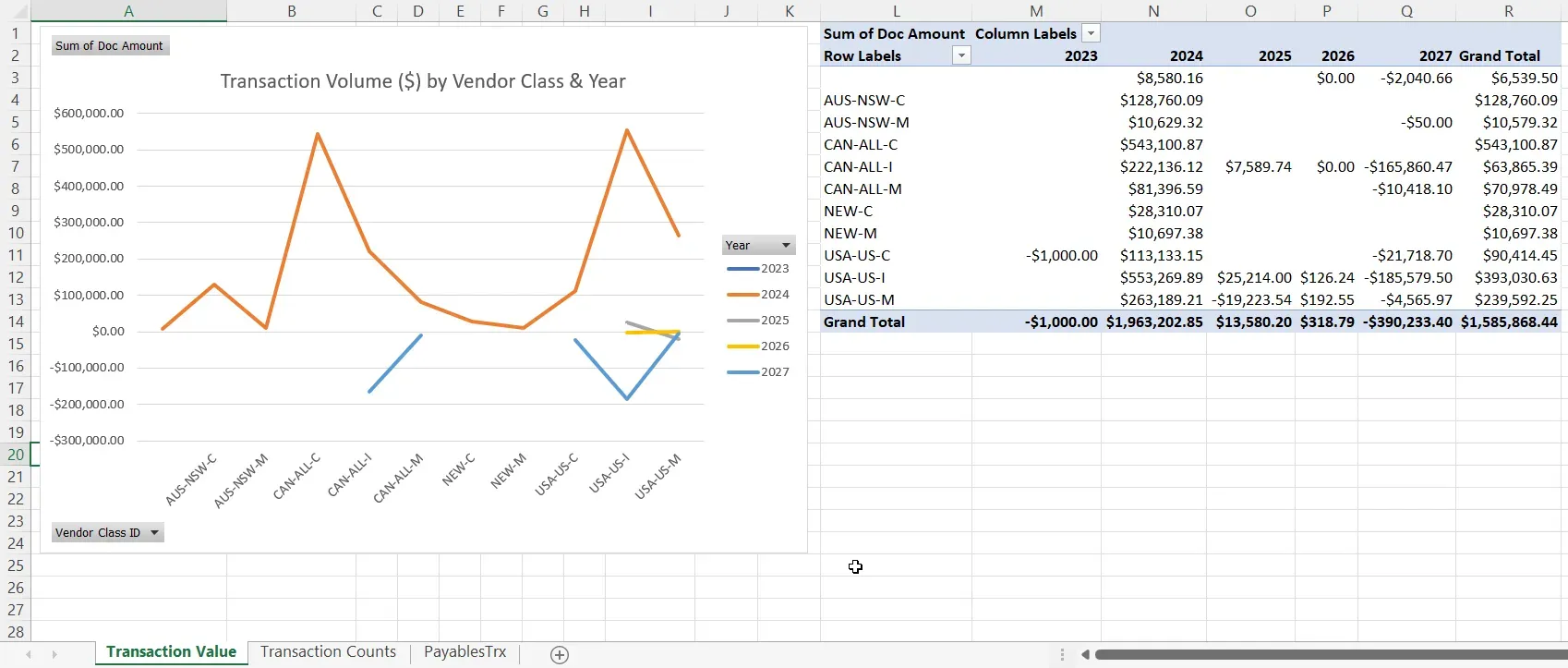
Example 1 - Line chart showing $ by Vendor Class & Year
This one is a Pivot Chart, a line chart, analyzing transaction dollars by year and vendor class.
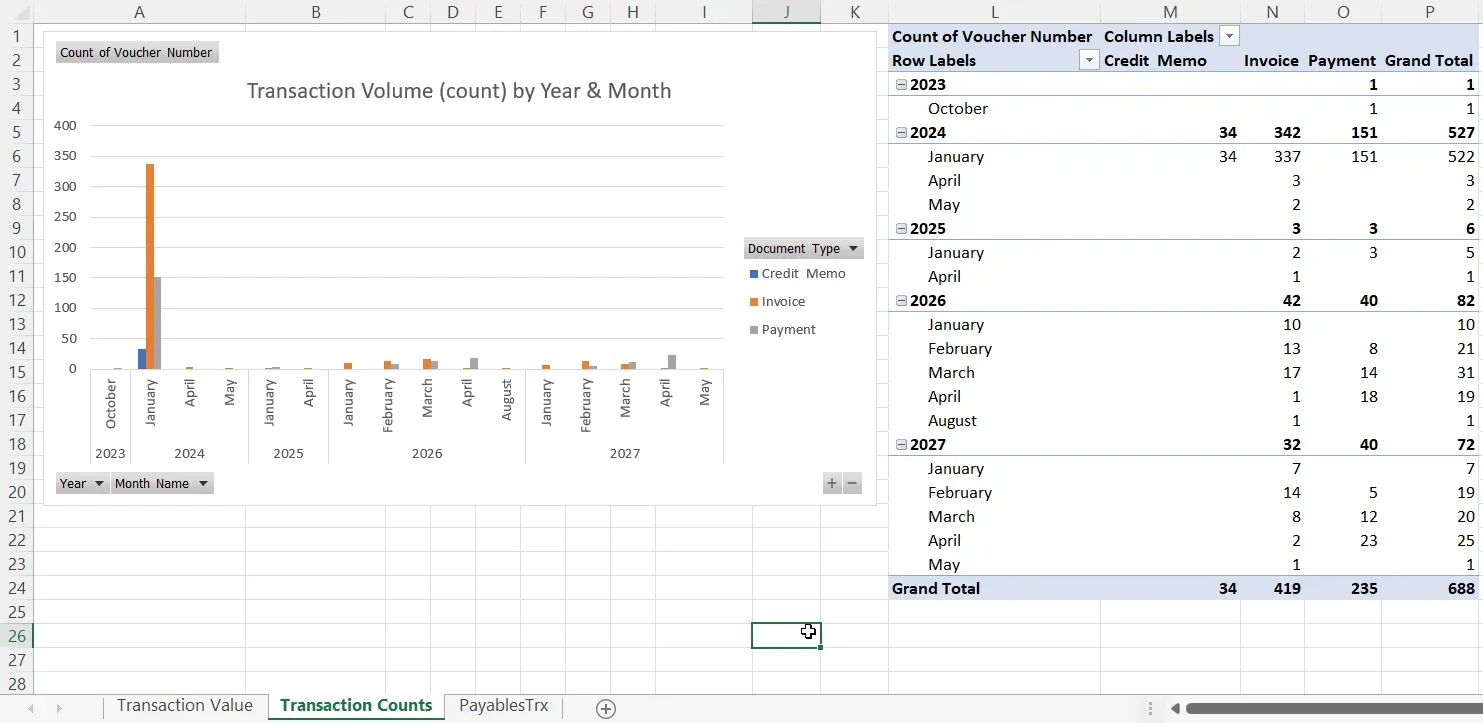
Example 2 - Column chart showing transaction count by Year, Month & Type
This one is a column chart analyzing transactions by document type and the count (number) of transactions.
Refresh won't work unless someone exported the same SmartList that I described above and changed the pathname etc., to the location where it was saved in the system.
That's it for this post. Hopefully, some of the basics here are useful as an introduction to Power Query. I've barely scratched the surface! Stay tuned for the next post in the series where I will talk about how to get the data out of GP via a connection to SQL.
