Today’s #TipTuesday is a detour from my recent SmartList tips for Dynamics GP, and I’m going back to Excel for this one.
I have been working on a project recently where some data validation is needed to ensure that user-entered data on some forms is valid. I want to have some visual validation for Accounting when reviewing these forms before uploading the data into Dynamics GP to determine in advance if the GL Accounts exist, or if the Job/Project and/or Cost Code/Category exists. In my use case, I can’t use the built-in Data Validation features as the lists would be too lengthy to be manageable, so the fields are simple text fields, prone to errors and typos.
I want an easy way to highlight invalid entries before proceeding further in the process, during the review stage. Specifically, I want to use Conditional Formatting to highlight anything that can be validated if it isn’t in various lists (of accounts, jobs, cost codes etc.).
My “old” method
For some reason, these types of queries in Excel give me a headache. Every time I run into this situation, I try a slightly different method and it always seems so convoluted. Historically I tend to go to VLOOKUP but it’s clunky (the way I’ve done it in the past). I end up with some IF and VLOOKUP or MATCH god-awful-looking formula that’s hard to troubleshoot.
A better way!
Today I had an “aha!” moment. I learned a new way to do this and it’s SO MUCH CLEANER! The simple tip is using COUNTIF to determine how many times a given value appears in a list. If it appears 0 times, it’s “missing” and needs to be highlighted or flagged. If it appears 1 or more times, it’s in the list.
Mind. Blown.
I could be the last person on the planet to think of this but honestly, it’s changed how I think about validation. (To be clear, I use conditional formatting all the time but I didn’t think of simply using COUNTIF to validate the existence of a value before… )
How to use this with Conditional Formatting
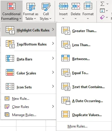
Conditional Formatting is a very powerful feature in Excel but is often intimidating to end users. It’s not always intuitive to set up if a user needs to do something outside of the canned examples (shown below).
In this example, I skipped the defaults and went into More Rules and the “Use a formula to determine which cells to format” option. Before I show this example, here is what my spreadsheet example looks like. It’s a Fabrikam Ltd. chart of accounts (Dynamics GP sample company) and off to the right is an example of two G/L Accounts, one valid, one not valid.
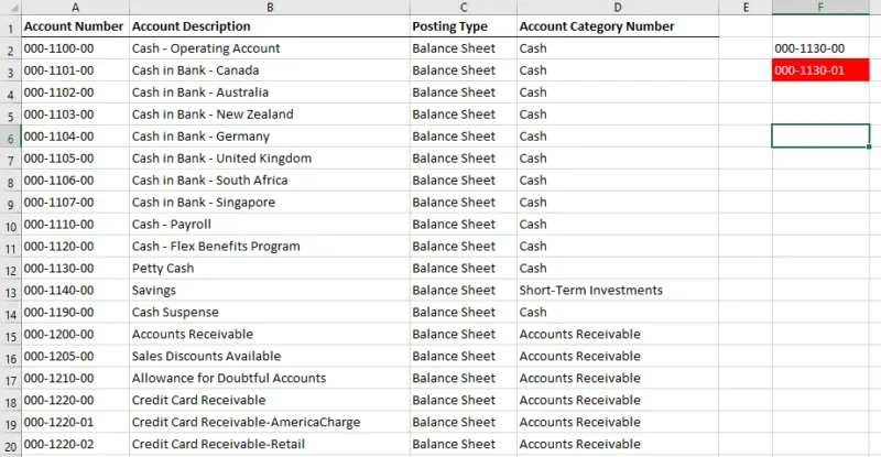
This example is simplistic, but in reality, I had a separate tab with a user-filled-out expense form and the conditional formatting is applied to any column where there was a GL Account entry option. In my example above, I simply want to check 2 accounts, in cells F2 and F3. I highlighted them, then went into Conditional Formatting > Highlight Cells Rules > More Rules > Use a formula to determine which cells to format.
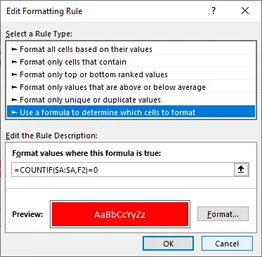
My formula is the COUNTIF formula I mentioned above. Here is where the syntax is weird in conditional formatting. I always read these as if the first equals sign isn’t there, because it looks weird right?
=COUNTIF($A:$A,F2)=0Two equals signs in a formula? Yeah… I agree. But, ignoring the first one makes the rest make more sense. Here’s how to read the formula and most importantly, how to get the absolute references correct.
- First, the formula I’m using is COUNTIF. I want to do a COUNTIF on the GL Accounts column in whatever list I have, i.e., count the instances of each account appearing. If they appear 0 times, the account is invalid.
- The first segment of the COUNTIF formula is the source to count, which is column A. This is an absolute reference (signified by the $ signs). No matter where my items are to be counted, it needs to “find” the account in column A, hence the absolute reference.
- The second segment of the COUNTIF formula is what to count. In this case, it’s F2, a non-absolute reference. If I made that absolute (“$F$2”), no matter what cell I applied to rule to, it would only look at the value of F2 to determine if the account is missing or not. I want it to look at F3 if it applies to F3, and I would want it to look at G3 if that’s where I was spot-checking a G/L Account too.
- Lastly, I want it to evaluate IF that COUNTIF is equal to 0, which is where the end of the COUNTIF formula, after the formula itself, has an “=0”.
Once I click OK (after setting my desired formatting), I am returned to this window below. This is where I tell Excel what cells this rule applies to.
Because F2 and F3 were highlighted when I clicked on conditional formatting in the first place, it applies to those 2 cells.
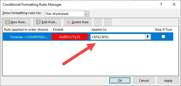
The result is the 00-1130-00 account is not formatted, because the COUNTIF would have resulted in a 1 for that account (it’s valid) but the 00-1130-01 account is invalid.
Summary
What’s beautiful about this approach is it’s much simpler to wrap my head around. If I use VLOOKUP or MATCH, I also need an IF and more than likely a wrapped like IFNA or IFERROR to catch the inevitable error when the thing I’m looking up is, in fact, not in the list in the first place. The formula becomes long and unwieldy.
I can’t believe I didn’t know about this tip before but I now know I’ll never forget it!