Today’s #TipTuesday is yet another Excel tip. I’ve been working with spreadsheets a lot lately. My blogs tend to follow my work and these last 3 weeks have been no exception. As I run into things or use something I haven’t touched in a while, I tend to blog about it!
This tip is about what I believe to be a hidden gem in Excel and that is the IFERROR formula. Over the years, I have seen many people do funky workarounds to “pre-check” if they will get an error when there is a formula that will help them out much more easily!
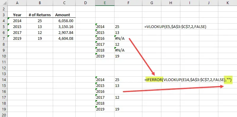
Example 1 – replace #N/A with blanks
The scenario I find it most useful in is in conjunction with something like a VLOOKUP formula. In my simple example, I am using the data from my blog last week with a few minor tweaks to introduce gaps in the years. The data is listing returns by year. In another area of my spreadsheet, I have a sequential list of years and want to find out the returns by year, and don’t know which years have data and which don’t.
In my first attempt, in the range E5 to F10, I have a basic VLOOKUP formula. What happens with VLOOKUP if there is no corresponding match to what I want to look up? It returns the #N/A error of course! If I have a subtotal at the bottom of this column of data, then suddenly one little error throws all of those formulas off too.
How to fix it
I like to describe IFERROR as a “wrapper” formula, as in, it is wrapped around the outside of anything else that could return an error I want to avoid. In my case, I want to put IFERROR and the opening bracket before my VLOOKUP formula, and then the first element is the VLOOKUP formula itself, then a comma, then the 2nd element which is “what do I want to show instead of the error?” (and then the closing bracket). In this example above, I chose an empty string, two double quotes to be specific, to show a blank in the cell if there is no data. The result is blanks for 2016 and 2018 where there were no returns.
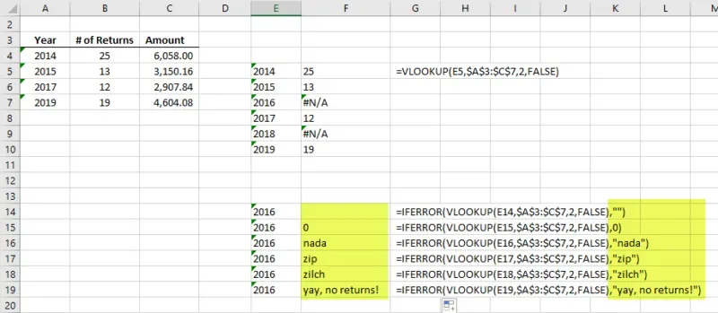
Other examples of replacement values
In the real world, this example might be more appropriate to have a numeric replacement, like a zero. Or, I might want a message there for a user, in case they expect a value to be there.
Using the same example from above, I had some fun with some alternate 2nd elements of the IFERROR formula to show several different options. Other than the last portion of the formula, the rest is identical and the VLOOKUP is just the normal syntax.
Recap
This is an enormously helpful yet simple formula that I use ALL THE TIME. It’s fantastic for VLOOKUPS but useful for other types of formulas too. I hope someone finds this useful!