Who has tried using a VLOOKUP formula in Excel to look up something numeric but stored as text, or vice versa? It’s annoying to have data formatted one way and the lookup in another. Today’s #TipTuesday is all about that, showing a couple of formula tweaks to make this a bit easier.
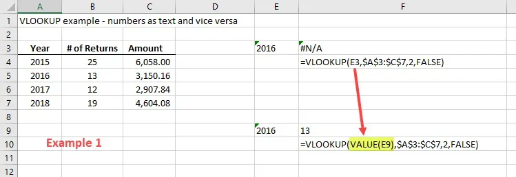
Example 1 – Text to Number
The first example is a small table where I’m looking up something by year, and the year is stored as a number in this case (column A). In cell E3, I have a year in text format (note the top left corner has the green mark, visually identifying this as text). If I do the usual VLOOKUP formula, I get an #N/A, it can’t find a match to that.
How to fix
In this case, I want to use the VALUE formula which is going to return the “value” of that cell, which is the number “2016”. With that small change, and the rest of the formula staying the same, it now returns the proper value I’m looking for (# of returns for a given year).
Old formula: (spaces are for readability only)
= VLOOKUP ( cell , array , column number , FALSE )New formula:
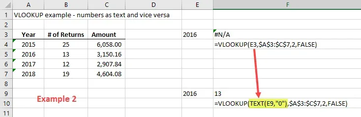
= VLOOKUP ( VALUE(cell) , array , column number , FALSE )Example 2 – Number to Text
The opposite scenario also happens regularly, where the list/array is in text format but the value I want to look up is a number. I’m using the same data as I did in Example 1, except now the year is stored as text (again, note the green visual indicator in Column A’s values). In cell E3, I have a year in number format. If I do the usual VLOOKUP formula, I get an #N/A, but I cannot use a VALUE( ) formula to fix this one.
How to fix
In this case, I want to use the TEXT formula to “convert” the value to a text format before using the VLOOKUP command. The TEXT formula has 2 elements to it, what the cell reference is and then the format I want. Here is a link to help with different format options (link) but in this case, the short version is if it’s a number, use “0” (zero) for the text format.
Old formula:
= VLOOKUP ( cell , array , column number , FALSE )New formula:
= VLOOKUP ( TEXT(cell, "0") , array , column number , FALSE )Recap
The short version of this tip would be: when it is not possible to make the data array and the value to be found in the same format (both numeric or both text), these are some easy ways to get the results relatively quickly and easily. The trick is changing the format of the thing the user is looking up, not changing the “array” of data the user is looking it up in!
Hopefully, that makes sense and saves some trouble in formulas!